LoRa and Projection to a Matrix Subspace

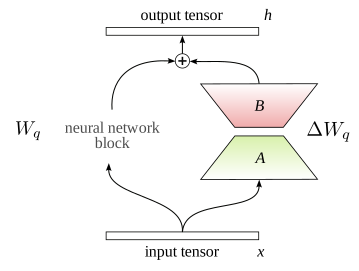
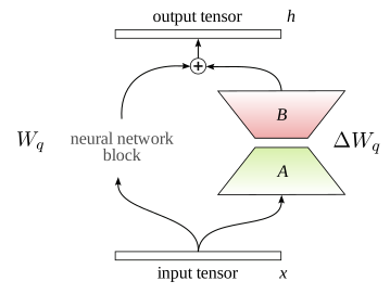
Low-Rank Adaptation technique was introduced to adapt large language models to a specific downstream task while keeping the original model intact and, by doing that, dramatically reducing the number of trainbale parameters. No only it lowers the hardware requirments to implement a task-specific adaptation but also it adds no inference latency when deployed.

Based on the assumption that pretrained language models have a low intrinsic dimension, authors constrain the update of a pre-trained weight matrix $ W_q \in \mathbb{R}^{d \times k } $ with a low-rank decomposition: $$ h = W_q x + \Delta W_q x = W_q x + B A x, $$ where $ B \in \mathbb{R}^{d \times r}, A \in \mathbb{R}^{r \times k}$ , and the adapted rank $ r \ll min\{ d, k \} $. In the paper they applied LoRa only to the attention weights of the Transformer architecture. This is why we see in the adaptation here a Transformer’s query matrix $W_q$.

To gain a deeper understanding of the relationship between the increment $ \Delta W $ and the original $ W $ matrices, it seems reasonable to project $W$, onto a subspace of $ \Delta W $ and to compute the Frobenius norm $ \| U^T W_q V^T \|_F $, where $ U $ and $ V $ are the left and the right singular-vector matrices of $ \Delta W $. Let’s see the reason behind this.

Suppose we have a matrix $ A $ with linearly independent comlumns. Then the projection matrix onto subspace of $ A $ would be:

$$ P = A(A^T A)^{-1}A^T. $$

In our case, if we want to project on the subspace of $ \Delta W_q $, we can express the projection matrix as (bearing in mind that SVD of $ \Delta W_q $ is $ U \Sigma V^T $): $$ \begin{split} P = \Delta W_q ( \Delta W_q^T \Delta W_q )^{-1} \Delta W_q^T = \\ U \Sigma V^T ( (U \Sigma V^T)^T U \Sigma V^T )^{-1} (U \Sigma V^T)^T = \\ U \Sigma V^T ( V \Sigma U^T U \Sigma V^T )^{-1} V \Sigma U^T = \\ U \Sigma V^T ( V \Sigma^2 V^T )^{-1} V \Sigma U^T = \\ U \Sigma V^T V^{-T} \Sigma^{-2} V^{-1} V \Sigma U^T = \\ U \Sigma \Sigma^{-2} \Sigma U^T = U U^T. \end{split} $$

And finally, the projection itself of matrix $ W_q $ is $ P W_q = U U^T W_q $ or $ U U^T W_q V^T V $, as matrix $ V $ is unitary, $ V^TV = I $.
As Frobenius norm is invariant under unitary operations $ U $ and $ V $ (follows from the cyclic nature of the trace), we can state that $ \| U U^T W_q V^T V \|_F = \| U^T W_q V^T \|_F $. From where comes the Feature amplificaiton factor mentioned in the paper:

$$ \frac{ \left \| \Delta W_q \right \|_F }{ \left \| U^T W_q V^T \right \|_F } $$ This factor demonstrates the interaction between subspaces and helps to understand what the adaptation is doing. For instance, experimental evaluation revealed that the matrix $ \Delta W $ amplifies singular directions that are not emphasized in the original matrix $W$ and the amplification factor is quite significant. It can be deduced from this that

the low-rank adaptation matrix potentially amplifies the important features for specific downstream tasks that were learned but not emphasized in the general pre-training model ¹.

Another tool that can shed light on the mechanics behind the adaptation is the measurement of similarity between subspaces with different adaptation ranks $ r $. This quantity can be calculated by using a normalized subspace similarity based on the Grassmann distance.

Suppose we have two adaptation matrices $ A_{r=8} $ and $ A_{r=64} $ with different ranks. Then we compute SVD for each of them and obtain the right singular matrices $ U_{r=8} $ and $ U_{r=64} $. The proposed in the paper similarity metric $ \phi $ helps to understand how much of the subspace spanned by the top $ i $ singular vectors in $ U_{r=8} $ is contained in the subspace spanned by top $ j $ singular vectors of $ U_{r=64} $:

$$ \phi(A_{r=8}, A_{r=64}, i, j) = \frac{ \| U_{A_{r=8}}^{iT} U_{A_{r=64}}^{j} \|_F^2 }{ min(i,j) }, $$

where $ U_{A_{r=8}}^i $ represents the columns of $ U_{A_{r=8}} $ corresponding to the top $ i $ singular vectors. This similarity metric resembles very much the well-known Projection metric which measures the distance between subspaces.

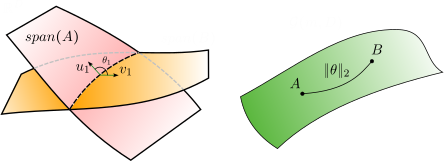
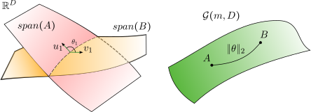
According to the definition, the Grassmann manifold $ \mathcal{G}(m,D) $ is a set of $ m $-dimensional linear subspaces of the Euclidean space $ \mathbb{R}^D $. Let’s take any two elements of the manifold $ \mathcal{G}(m,D) $ — the orthonormal matrices $ A $ and $ B $ of size $ (D \times m) $. In the same time $ span(A) $ and $ span(B) $ represent two subspaces in $ \mathbb{R}^D $. The distance between two subspaces $ span(A) $ and $ span(B) $ can be measured using the pricipal angles $ [\theta_1, \dots, \theta_m] $ as the usual dot-product of vectors. In the Grassmann manifold however, these two subspaces are represented simply by two points and the Riemannian distance between them is simply $ d(A, B) = \| \theta \|_2 $.
The set of principal angles $ 0 \le \theta_1 \le \dots \le \theta_m \le \pi/2 $ between two subspaces $ span(A) $ and $ span(B) $ are defined by $$ cos \theta_k = \max_{u_k \in span(A)} \max_{v_k \in span(B)} u_k^Tv_k. $$

where $ u_k $ spans $ A $, $ v_k $ spans $ B $ and $$ \begin{split} u_k^T u_k = 1, v_k^T V_k = 1, \\ u_k^T u_i = 0, v_k^T v_i = 0, ( i = 1, \dots, k-1 ). \end{split} $$

In other words, the first principal angle $ \theta_1 $ is the smallest angle between all pairs of unit vectors in the first and the second subspaces ².

To compute these principal angles we need to find the SVD of $ A^TB $:

$$ A^TB = U diag(\sigma_1, \dots, \sigma_m) V^T = U(cos\Theta)V^T, $$

where $ U = [u_1, \dots, u_m], V = [v_1, \dots, v_m] $ and $ cos\Theta $ is the diagonal matrix $ cos \Theta = diag(cos\theta_1, \dots, cos\theta_m ) $.
Another popular expression of a distance betwen subspaces is the Projection Metric (2-norm of the sine of principal angles): $$ d_P(A,B) = \left ( \sum_{i=1}^m sin^2 \theta_i \right )^{1/2} = \left ( m - \sum_{i=1}^m cos^2 \theta_i \right )^{1/2} = \left ( m - \sum_{i=1}^m \sigma_i^2 \right )^{1/2}. $$

Let’s return to the similarity metric $ \phi $. If the singular values of the product $ U_{A_{r=8}}^{iT} U_{A_{r=64}}^j $ are $ \sigma_1, \sigma_2, \dots, \sigma_p $, where $ p = min(i,j) $, then the similarity is defined as:

$$ \begin{split} \phi(A_{r=8}, A_{r=64}, i, j) = \frac{ \| U_{A_{r=8}}^{iT} U_{A_{r=64}}^{j} \|_F^2 }{ min(i,j) } = \\ = \frac{ \sum_{i=1}^{p} \sigma_i^2 }{p} = \frac{1}{p} \left ( 1 - d_P( U_{A_{r=8}}^{iT}, U_{A_{r=64}}^{j} ) \right ), \end{split} $$ which is exactly a reverse of the Projection Metric defined earlier.

Using this similarity metric and having carried out multiple experiments the authors concluded

that the top singular-vector directions of $ A_{r=8} $ and $ A_{r=64} $ are the most useful, while other directions potentially contain mostly random noises accumulated during training. Hence, the adaptation matrix can indeed have a very low rank ¹.