Stereo Transformer & Sinkhorn Iterations

Revisiting Stereo Depth Estimation from a Sequence-to-Sequence Perspective with Transformers¹.

This may seem like an outdated paper from prehistoric 2021, especially in the contemporary high-speed deep learning race, but it’s full of original ideas:

• Using transformer’s cross-attention for stereo matching without restriction to a disparity range and without the need for constructing highly memory-demanding discrete cost volumes.
• Clever use of entropy-regularised optimal transport to impose a uniqueness constraint on disparity with the elegant differentiable Sinkhorn algorithm.
• No finite and fixed discrete disparity values, instead a dense continuous disparity function allowing for a sub-pixel resolution.
• Naturally handles occlusions by using a learnable parameter to assign the cost of an unmatched pixel.

Let’s scratch a little bit on the surface of the theory of optimal transport and see how it came to be useful in the modern deep learning workflow.

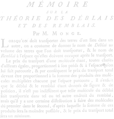
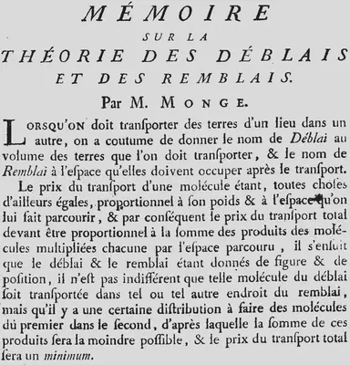
The optimal transport problem originated from Gaspard Monge’s 1781 paper on the optimality of moving a pile of dirt from one place to another. It minimises the total work required, taking into account the transportation cost, which is determined by the amount of mass moved and the distance taken:

This formulation is a special case of the optimal transport problem where the cost of transportation is given by Euclidean distance. It is commonly referred as Earth Mover’s Distance.

Sometimes we need to measure the distance between two distributions ( $ \pi $ and $ p $ ), for example in GANs or variational autoencoders.

For this purpose we already have a well known family of $ f $-divergencies $ D_f(\pi || p) = \mathbb{E}_{p(x)} f\left ( \frac{\pi(x)}{p(x)} \right )$, Kullback–Leibler or Jensen-Shannon to name a few. But for disjoint manifolds or distributions with disjoint supports they no longer represent a feasible distance as $ KL(\pi ||p ) = \infty $ and $ JSD(\pi || p) = \log(2) $, let alone proper gradient propagation.

Another application might be interpolation between distributions, where we can find a smooth transition expressed in barycentric coordinates:

Suppose we have two descrete distributions of size $ n $ and a cost matrix $ \mathbf{C} \in \mathbb{R}^{n \times n} $. Gaspard Monge’s optimal assignment problem looks for a mapping that associates to each point $ x_i $ a single point $ y_i $ or in other words it attempts to find a bijective function $ \sigma $ in the set of permutations of $ n $ elements to minimize:

This formulation of optimal assignment has some drawbacks: the problem itself is nonconvex, it may have several optimal solutions and sometimes a feasible solution does not exist. To overcome these inconveniences Kantorovich proposed to relax this deterministic nature of assignment. Originally a source point $ x_i $ can only be assigned to another point $ y_{\sigma_i} $, but Kantorovich suggested instead that the mass at any point $ x_i $ can be potentially dispatched across several locations or it can be splitted from a source towards several targets. This relaxation allows, in place of permutations $ \sigma $, to use a transportation matrix $ \mathbf{P} \in \mathbb{R}^{n \times m}_{+} $:

where $ \mu, \nu $ — discrete measures with weights $ a_i, b_j $ at locations $ x_i, y_j $; $ \delta_x, \delta_y $ — Dirac functions; $ \mathbf{a}, \mathbf{b} $ — marginal source and target distrubutions; $ \mathbf{C} $ — a transporatation cost matrix or a matrix of pairwise distances; $ \mathbf{P} $ — a transportation plan matrix we are looking for, with a constraint that its columns and rows sums should match marginals.
$ P_{i,j} $ describes the amount of mass flowing from location $ i $ to location $ j $.

It looks like a linear program, so there must exist a dual which was formulated by Kantorovich (probably furnished him the Nobel Prize in economics):

Here we are looking for optimal dual variables $ \alpha, \beta $ (Kantorovich potentials). We can write the Lagrangian of the primal problem:

After exchanging the min and the max we obtain:

We can observe that for any $ \mathbf{Q} $:

so that the constraints definetely are $ \mathbf{C} - \alpha \mathbb{1}_m^{\mathrm{T}} - \mathbb{1}_n \beta^{\mathrm{T}} \ge 0 $ or $ \alpha_i + \beta_j \le \mathbf{C}_{i, j} $.

Returning to the original problem, we can see that the set of matrices $ \mathbf{U} ( \mathbf{a}, \mathbf{b}) $ is defined by $ n+m $ equality constraints that form a convex polytope of feasible solutions with a cost vector $ \mathbf{C} $ and the optimal solution $ \mathbf{P}^{\star} $ located at a vertex:

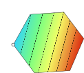
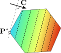
The problem could be solved with a network flow solver with $ O(n^3log(n)) $ complexity². But unfortunately, this solution is not differentiable on discrete inputs, making it unsuitable for use in a deep learning pipeline. To complicate things more, the solution $ \mathbf{ P } ^{\star} $ is not stable upon small changes in the input distrubutions and not always unique when the cost vector $ \mathbf{C} $ is orthogonal to a face of the polytope:

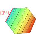
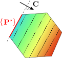
To address these inconveniences, sacrifices must be made and the particular one is giving up on the exact solution.

The idea of the entropic regularization of optimal transport is to use the entropy of the transport matrix as a regularisation function to obtaine an approximate solution to the original problem³.

where

is the discrete entropy of the transport matrix, $ \gamma $ — determines the extent to which entropy influences the solution.

This augmented objective function has a solution which is no longer located on a vertex of the polytope. The entropy term pushes the original solution away from the boundary to the regularized entropic minimum. You can see the impact of increasing $ \gamma $ on the cost landscape of the linear problem:

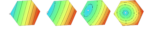
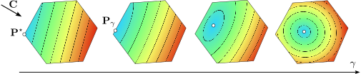
Formally the unique solution converges to the optimal one with the maximum entropy:

In the edge cases, when $ \gamma \rightarrow 0 $, it converges to the linear program solution:

and for a large regularization $ \gamma \rightarrow \infty $, the solution converges to the joint probability between two independent random variables distributed according to marginals $ \mathbf{a} $ and $ \mathbf{b} $:

A natural way to solve a constrained minimization problem is to make a Lagrangian:

After having assigned derivatives over components $ P_{i,j} $ to zero, we can express the solution for $ \mathbf{P} $:

If we assume:

we can rewrite the expression in a vector form:

$ \mathbf{K} $ is called Gibbs kernel and $ \mathbf{u}, \mathbf{v} $ are Sinkhorn scalings.

Let’s use the normalization constraints $ \mathbf{P} \mathbb{1}_m = \mathbf{a}, \mathbf{P}^{\mathrm{T}} \mathbb{1}_n = \mathbf{b} $:

or simpler:

where $ \odot $ is Hadamard product. Solving this for $ \mathbf{u} $ and $ \mathbf{v} $ gives us an iterative solution know as famous Sinkhorn algorithm⁴ with $ O(nm) $ complexity⁵:

where $ \oslash $ stands for an element-wise division.

We can see the impact of the regularzation parameter $ \gamma $ on the solution, wich behaves like a temperature:

If we let the temperature approach zero, we approximate the exact solution. Conversely, if we let $ \gamma $ go to infinity, the solution is just an outer product of the two marginal distributions.
So Sinkhorn procedure involves a sequence of vector matrix multiplication that is perfectly differentiable. This allows it to be used within a neural network, taking advantage of GPU acceleration and PyTorch auto-differentiation.

And this is a suitable place to return to Stereo Transformer paper.
The achitecture of the network consists of a feature extractor backbone, a bunch of self- and cross-attention Transformer blocks and finally, a regression head with the Context Adjustment Layer:

The optimal transport finds its place in the last transformer’s cross-attention block and it is replacing the Softmax operator usually used in the Transformer achitecture.

The optimal transport problem is formulated as follows:

• The cost matrix $ \mathbf{C} $ is set to the negative cross-attention. Softmax is not used as optimal transport normalizes the attention values.
• The two marginal distributions $ \mathbf{a} $ and $ \mathbf{b} $ are uniform, which imposes a soft uniquness constraint and mitigates ambiguity.

If the two marginal distribution have equal length and $ \mathbf{a} = \mathbf{b} = \mathbb{1}_n / n $, then the optimal assignment problem becomes the optimal matching problem and there exists an optimal solution $ \mathbf{P}_{\sigma^{\star} } $, which is a permutation matrix associated to an optimal permutation $ \sigma^{\star} \in \mathrm{Perm}(n) $³.

Additional boilerplate is done to add a learnable dustbin $ \phi $ responsible for unmached occluded pixels. The intuition behind the optimal transport solution $ \mathbf{P} $ is that entries $ P_{i,j} $ could be interpreted as pair-wise pixel matching probabilities.

Let’s examine the code and analyse how it was implemented:

def _optimal_transport(self, attn: Tensor, iters: int):
    """
    Perform Differentiable Optimal Transport in Log-space for stability
    Adapted from SuperGlue (https://github.com/magicleap/SuperGluePretrainedNetwork)

    :param attn: raw attention weight, [N,H,W,W]
    :param iters: number of iterations to run sinkhorn
    :return: updated attention weight, [N,H,W+1,W+1]
    """
    bs, h, w, _ = attn.shape

    # set marginal to be uniform distribution
    marginal = torch.cat([torch.ones([w]), torch.tensor([w]).float()]) / (2 * w)
    log_mu = marginal.log().to(attn.device).expand(bs, h, w + 1)
    log_nu = marginal.log().to(attn.device).expand(bs, h, w + 1)

    # add dustbins
    similarity_matrix = torch.cat([attn, self.phi.expand(bs, h, w, 1).to(attn.device)], -1)
    similarity_matrix = torch.cat([similarity_matrix, self.phi.expand(bs, h, 1, w + 1).to(attn.device)], -2)

    # sinkhorn
    attn_ot = self._sinkhorn(similarity_matrix, log_mu, log_nu, iters)

    # convert back from log space, recover probabilities by normalization 2W
    attn_ot = (attn_ot + torch.log(torch.tensor([2.0 * w]).to(attn.device))).exp()

    return attn_ot

• The iterative process is done in logarithmic space for better numerical stability.
• The two marginals $ \nu $ and $ \mu $ are initialized as log of the uniform distribution.
• The shape of the attention tensor is [bs, n, h, w, w], the shape of marginals is [bs, h, w + 1], the last value here is for the dustbin $ \phi $.
• All the values in the range [1:w] are initialized to 1/(2*w) and the last value is 0.5, so the whole distribution sums up to 1. Increased weight on the dustbin here is for balancing out its influence with the disparity bins.

    # set marginal to be uniform distribution
    marginal = torch.cat([torch.ones([w]), torch.tensor([w]).float()]) / (2 * w)
    log_mu = marginal.log().to(attn.device).expand(bs, h, w + 1)
    log_nu = marginal.log().to(attn.device).expand(bs, h, w + 1)

Then a similarity_matrix (optimal transport matrix) is constructed by adding the learnable dustbin phi to the last row and column of the attention tensor:

    # add dustbins
    similarity_matrix = torch.cat([attn, self.phi.expand(bs, h, w, 1).to(attn.device)], -1)
    similarity_matrix = torch.cat([similarity_matrix, self.phi.expand(bs, h, 1, w + 1).to(attn.device)], -2)

phi is a learnable scalar parameter previously defined in the constructor:

    self.phi = nn.Parameter(torch.tensor(0.0, requires_grad=True))  # dustbin cost

The last step is to run a few Sinkhorn interations and recover the transport matrix by exponentiation. Number of iterations is set to 10:

    # sinkhorn
    attn_ot = self._sinkhorn(similarity_matrix, log_mu, log_nu, iters)

    # convert back from log space, recover probabilities by normalization 2W
    attn_ot = (attn_ot + torch.log(torch.tensor([2.0 * w]).to(attn.device))).exp()

Let’s look into _sinkhorn method:

def _sinkhorn(self, attn: Tensor, log_mu: Tensor, log_nu: Tensor, iters: int):
    """
    Sinkhorn Normalization in Log-space as matrix scaling problem.
    Regularization strength is set to 1 to avoid manual checking for numerical issues
    Adapted from SuperGlue (https://github.com/magicleap/SuperGluePretrainedNetwork)

    :param attn: input attention weight, [N,H,W+1,W+1]
    :param log_mu: marginal distribution of left image, [N,H,W+1]
    :param log_nu: marginal distribution of right image, [N,H,W+1]
    :param iters: number of iterations
    :return: updated attention weight
    """

    u, v = torch.zeros_like(log_mu), torch.zeros_like(log_nu)
    for idx in range(iters):
        # scale v first then u to ensure row sum is 1, col sum slightly larger than 1
        v = log_nu - torch.logsumexp(attn + u.unsqueeze(3), dim=2)
        u = log_mu - torch.logsumexp(attn + v.unsqueeze(2), dim=3)

    return attn + u.unsqueeze(3) + v.unsqueeze(2)

Firstly vectors $ \mathbf{u} $ and $ \mathbf{v} $ are zero initialized. Then the cost matrix $ \mathbf{C} $ is set to the negative attention attn, which is intuitively understandable: the most attended pixels have the least transportation cost. The regularization parameter $ \gamma = 1 $.

With these assumptions in mind we can rewrite the kernel $ \mathbf{K} $ as:

Plugging this kernel into the Sinkhorn update and taking log of the equality, we achieve the original expression:

This conсludes the matter. It is worth mentioning that in the ablation studies section, it was demonstrated that the soft uniqueness constraint imposed by optimal transport improved all the metrics: end-point-error (EPE), 3px error and occlusion IOU.

Finally, I would like to express my gratitude to the authors for their outstanding work and for providing a clear example of how Optimal Transport can effectively complement existing deep learning techniques.